Integration By Parts

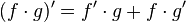
Integration By Parts - this is a method for solving integrals involving products of functions. By products of functions we mean:

f(x)g(x), or xCos[x], where x is a function and Cos[x] is a function. Here is the parts formula:

Now, you might wonder how this was derived...well, this is derived from the product rule. Recall the product rule for differentiation:

If this isn't making sense yet don't worry. What you need to realize is that the integral of the left side of the above equation, is simply f*g. Remember that the integral of a derivative, is just a function. Quickly:

f(x) = x^2
f '(x) = 2x
Integral of 2x = (2 *x^2)/2, and the 2s cancel leaving us with x^2 or f(x).

So, since the left and right side of any equation are equivalent :-), we can also integrate the right side of the equation. After recalling the fact above, that the derivative of an integral is just the function and a little rearranging we arrive at the integration by parts formula. Look at the below.

• First is the product rule
• Then you integrate the derivative to get back the original f(x)*g(x) function.
• Then you rearrange the equation...that's it.

(note, in the first line, that's g ' (x), ignore the carrot, there is no exponent)

Let's do a integration by parts problem:

Notice here, U substitution doesn’t work. There’s no trig substitution to fall back on and there is no immediately obvious antiderivative.

Let’s use integration by parts, note, we will be replacing f and g with u and v, don’t get too excited!

So how do you choose u and v? Good question, let’s think about it for a second. Looking at the integration by parts formula, you have to take the antiderivative of u on the right side of the equation. The goal is always to get a simpler integral on the right side of the equation. So if differentiating u creates a integral more complicated than the original integral on the left, don’t use it.

Note that we choose u, lnx so that it's derivative is easy to integrate, it happens to cancel nicely with the antiderviate of dv, so enjoy that while you can.

So we have our answer, the indefinite integral is highlighted. Note, a few principles used in the simplification included reducing the power of the exponent and eliminating the x in the denominator, and bringing out a constant in front of the integral.

Also - in case that wasn't enough (I doubt it), some great videos on integration by parts on YouTube. And if you like cheap books, check out th

e iChapters ad on the right. You can buy individual chapters, in PDF format for a few bucks a piece...that's a cool deal!

So we have our answer, the indefinite integral is highlighted. Note, a few principles used in the simplification included reducing the power of the exponent and eliminating the x in the denominator, and bringing out a constant in front of the integral.

Daily Problem Emailed

Buy ONLY The Chapters You Need For Class - Not The Whole Book! All digital and CHEAP.

Chebyshev's inequality + Examples

Chebyshev's inequality:In very common language, it means that regardless of the nature of the underlying distribution that defines the random variable (some process in the world), there are guaranteed bounds to what % of observations will lie within K standard deviations of a mean.

So you need the following:

- Mean of the probability distribution
- Standard deviation or variance of the distribution, recall that variance is stdev^2

Let's do a simple example:

The length of a knife is on average 5 inches long, with a standard deviation of 1/10th of 1 inch. What % of observations will be between 4.75 and 5.25 inches long? We can approach this several ways, but let us take the most intuitive route:

The mean is 5 inches...so we're trying to find how often knives will be within 1/4 inch on either side of the mean. Now, if a knife is 5.25 inches, how many standard deviations is the length off by? Recall that our standard deviation is .1 inches. So, .25 inches/.1inch = 2.5 standard deviations. Note that this means that:

mean +/- 2.5 standard deviations = the range of lengths 4.75 to 5.25 inches.

Now we can solve the problem:

Let's think about this statement. It says the chance that the absolute difference between the observed length and the mean is greater than k standard deviations (k is arbitrary, it could be anything), is equal to 1/k^2. Now k is the # of standard deviations.

So this gives the probability that the observation will be GREATER than k standard deviations. We are trying to find the probability that it's on some interval namely, 4.75 to 5.25 inches. So, if the above is P(A), than the probability we want is 1-P(A).

So let's do it:

1 - 1/k^2 = 1-1/2.5^2 = 1 - 1/6.25 = 1-.16= 84% (.84 = 84%).

So, that's it. Keep in mind this assumes that the MEAN IS KNOWN and the VARIANCE OR STDEV IS KNOWN. If those are not known, you can't use this. And for completeness, what is the probability that the knives observed will be off the 4.75 inch to 5.25 inch interval?

Well, it's just 1-P(that they're on the interval) so 1-84% = 16% OR, and I hope you're thinking about this already, 1/2.5^2 = 1/6.25 = 16%. So that odds that they are either ON or OFF the interval, the union of 2 mutually exclusive events is just their sum, 84%+16% = 100%.


Wikipedia on the subject:

In probability theory, Chebyshev's inequality states that in any data sample or probability distribution, nearly all the values are close to the mean value, and provides a quantitative description of "nearly all" and "close to".

In particular,

* No more than 1/4 of the values are more than 2 standard deviations away from the mean;
* No more than 1/9 are more than 3 standard deviations away;
* No more than 1/25 are more than 5 standard deviations away;

and so on. In general:

* No more than 1/k2 of the values are more than k standard deviations away from the mean.

Let X be a random variable with expected value μ and finite variance σ². Then for any real number k > 0,

Only the cases k > 1 provide useful information. This can be equivalently stated as

As an example, using k = √2 shows that at least half of the values lie in the interval (μ − √2 σ, μ + √2 σ).

Typically, the theorem will provide rather loose bounds. However, the bounds provided by Chebyshev's inequality cannot, in general (remaining sound for variables of arbitrary distribution), be improved upon. For example, for any k > 1, the following example (where σ = 1/k) meets the bounds exactly.

For this distribution,

A one-tailed variant with k > 0, is

Daily Problem Emailed

Buy ONLY The Chapters You Need For Class - Not The Whole Book! All digital and CHEAP.

Natural Logarithm as An Integral

Today we'll look at the natural logarithm lnx as an integral. Let's first consider the function ln(x), which is the natural logarithm of x. d/dx ln(x) = 1/x, so we can say that the integral of ln(x) from 1 to x is the value of ln(x) at x, because ln(x) at x = 1 is 0. Here's a better visual. Pay attention to the black writing in the top right of the image.

Again, this simply states that the antiderivative or definite integral of 1/x is the natural logarithm of x. Here note that as this is a definite integral there are limits of integration, namely 1 and x...so be sure to realize that the end limit of integration is varying in this case and can take on any value so long as it's greater than 1. If it's less than 1, (x < ln2 =" .693."> 2 is just ln(2).

You'll see in the first image that I've also computed the area under the curve from .5 to 1. It happens to be exactly the same as the area from 1 to 2, but if you compute the natural logarithm of .5 you'll get -.693, thus requiring you to keep in mind that although the sign of the result is negative, the area is most certainly positive.

So there you go, a simple example of the natural logarithm as an integral of 1/x. Keep in mind integration and differentiation are reverse processes. You were given a function and were asked to the area under it on an interval. You took the integral (or antiderivative) of the function and although we neglected to mention it, you took the difference of the limits of integration evaluated using the integral of 1/x - we ignored Ln(1) as it equals zero - but to be formal.

Integral of 1/x = Ln(x) | Area between 1 and 2 equals Ln(2) - Ln(1) = Ln(2) = .693.

This practice is derived from the fundamental theorem of calculus:

.

Then

Here's a great video on the fundamental theorem if you'd like to brush up/learn more about it.

Daily Problem Emailed

Buy ONLY The Chapters You Need For Class - Not The Whole Book! All digital and CHEAP.

Integral Mean Value Theorem & Mean Value Theorem

Today we'll explore the integral mean value theorem along with the mean value theorem for differential calculus. They're very similar in concept and will be fundamental in proving the Fundamental Theorems of the Calculus.

Mean Value Theorem -

If f(x) is continuous on the closed interval [a,b] and differentiable on the open interval (a,b) - there's at least 1 point "c" between a and b where

the derivative of c is equal to the slope of the secant line between a and b. Now, said that way you might be thinking to yourself, "what's the big deal." Fair enough. Let's take a look at a visual representation made in Mathematica:


What this means is that if the condition of f being continuous over [a,b] and differentiable over (a,b) there must be some C such that a where f '(c) = m of the secant line between AB.

The secant line is the average derivative of the curve over the interval. At least one time the derivative at a point will = the average derivative.

So - you're speeding along in your Ferrari for an hour. You end up driving 145 miles from point A to point B in an all out sprint (not shown). Can you guarantee that for at least 1 instant (perhaps more but at least for an infinitesimally small quantity of time you did go 145mph? You sure can. The mean value theorem guarantees that over a curve (the drive), your instantaneous velocity (f prime of c) must be equal to your average speed (secant line) at some point.

Integral Mean Value Theorem -

Given a function f(x) that's continuous over [a,b] there exists some c such that a <>

Said differently - f(c)*(b - a) equals the area beneath f(x) from a to b. Stated even more plainly, if you choose the right C, the area of the rectangle that you create whose height is f(c) and width if [a,c] will = the area under the curve. Here's an illustration done with Mathematica.

In this case, the gold rectangle with base 2.88-0 and height f(c) has area equal to the curve f(x) over the interval a to b.

Let's examine another image and see what this graph would look like had we chosen a value for C greater than ~2.88.

Clearly the area of the rectangle when using c = 4 results in an area that nearly doubles the area under the curve.

So the C you choose - is a function of the function and the mean value theorem for integration simply guarantees that there will be some C, where the area of the rectangle will equal the integral (area under f(x)) - just as in the above example for the mean value theorem used in differential calculus, there was some derivative of f(x) at c between [a,b] where the instantaneous slope was = average slope of the function.

Sign up for the daily email if you'd like. Check out the banner on the right too, iChapters let's you buy only the chapters you need. The whole chapter on integration in Stewart Calculus is under $8.00! That's not too shabby.

Resources:
Wolfram Integral Mean Value Theorem + Mean Value Theorem

Daily Problem Emailed

Buy ONLY The Chapters You Need For Class - Not The Whole Book! All digital and CHEAP.

Differentiate Using Chain Rule Twice

Today we'll do a simple problem. Plain old differentiation using the chain rule but we'll have to apply it multiple times. Here's the problem:


Cos(x^3)^2 written differently. Keep in mind this isn't a product and we can't employ the product rule here. If you'd like to review the product rule however there's a link to a short video tutorial on the product rule at the end of this entry.

Recall that the chain rule is as follows:

In this case our f(x) is cos^2(x) and our g(x) is x^3. Let's begin to differentiate:

2*cos(x^3)*-sin(x^3)*3x^2 - here's the image of what I've written to the left -

Let's think about this - we used the power rule to get the exponent in front of the cos(x)

power rule

Then you multiply the 2 by the inside of the balance of the functions. Then you take the derivative of the cos, which yields -sin, followed by the derivative of x cubed by itself. The final answer is a product of each successive differentiation.

.
So remember - when using the chain rule more than once remember to keep differentiating the outer part of the expression and work your way inward, multiplying by the results of your differentiation to arrive at the final answer.

Here's a good video on the product rule - remember that the quotient rule is just the product rule in disguise and sometimes it's better to take a quotient and create a product through use of a negative exponent.

Daily Problem Emailed

Buy ONLY The Chapters You Need For Class - Not The Whole Book! All digital and CHEAP.

Area Under a Curve as Limit - Find The Function

This problem involves analyzing the limit of the approximating rectangles which tells us the area under a curve, and determining what the function is along with what interval we're measuring area under.

Here's the limit:




How do we find the function and the interval whose area is described by the above limit? Well, we know that the area of a rectangle is

height * base -- so it follows that the area of an approximating rectangle under a curve is just the width of the interval * f(x) evaluated at the chosen endpoint/midpoint. Here's a graph to refresh your memory.


In this particular illustration, they are creating the approximating rectangles using the left endpoints. You can tell because the horizontal lines are being drawn from x = a which is the leftmost endpoint on the interval.

Also note that when a function is increasing over an interval, using left endpoints will underestimate the area under the curve. Using right endpoints will force an overestimate for the same function.


So the area of the first rectangle is b-a/7 (effectively the width of the rectangle) * f(Xa).

Back to the question:


Recall that this is a summation formula and if you look at the term outside the parentheses there is a term that will be distributed through the set of terms being influenced by the "i" in the limit. 2/n represents the width of the interval for each approximating rectangle. So this is the base of the rectangle. If you're wondering which rectangle remember this - 2/n is a constant proportion representing the area of any given rectangle. If we had 1000 rectangles that width would be 2/1000. Don't think of the width of the approximating rectangles as varying from rectangle to rectangle.

So b-a/n = 2/n. This means that the difference between b and a is 2. Without knowing anything else we could guess that the interval is 45 to 47, or 87 to 89. It's not right but at least the distance of the interval would be accurate. The area would be a bit high I'm afraid though.

So let's figure out what A and B are. The term in the parentheses represents the function evaluated at the Xi at the ith subinterval. It's 5 + 2*something/n. The 5 tells us something - it tells us that the interval begins at x = 5.

So a = 5, which means that if b - 5 = 2, b = 7.

The function turns out to be f(x) = x^10 and on the interval [5,7].

Considering the term in the parentheses, it's simply describing the height of the approximating rectangle at the ith subinterval in a generalized way. As the term 2/n is just describing the interval in a generalized way.

Daily Problem Emailed

Buy ONLY The Chapters You Need For Class - Not The Whole Book! All digital and CHEAP.

Sigma Notation Summation Rules & Limits at Infinity

Let's review the basic summation rules and sigma notation to find the limit of a sum as n approaches infinity. First let's review the basic rules and then we'll get to the problem - which is a problem you'd generally see preceding a discussion of the definite integral.

Recall that the "n" on top of the Sigma (the funny looking e) is the terminal value for the index which is located under the sigma. Note that the i= "something" tells you where to begin the summation.

1) Rule one states that if you're summing a constant from i=1 to n, the sum is equal to the constant multiplied by n. This makes intuitive sense. If i=1, and n = 100, and C was 1, 1(100) = 100.

2) Rule two states that the sum of increasing integers is simply n(n+1)/2. We'll leave the proof for another time but for now we can have faith in its utility.

3) Rule 3 states that the sum of increasing squared integers is equal to the formula.

4) Rule 4 is the same as rule 3 but handles the sum of increasing cubed integers.

Now let's evaluate the limit of a summation as n approaches infinity. Here's the problem:


One of the first considerations we need to make is what isn't affected by i, or what term(s) doesn't need a summation rule to be applied to it? First let's collect all terms outside of the parentheses and then square the inside term. After we've set this up we can apply the summation formula to all the terms inside the parentheses. Here are the steps.

Now we have to evaluate each term. We know from rule 1 above, the sum of a constant is simply c*n. So this will just be n. The middle term will be 2/n* the rule above which handles the sum of increasing integers n(n+1)2. The third term is a bit tricker - we take a 1/n^2 and place it to the left of the Sigma and evaluate i^2, whose rule is listed above. Here's the result visually:





Now we'll simplify through algebraic manipulation and distribute in the 3/n.


We see that in the 3rd image to the left that the 6 will remain, the 2nd term gets wiped out, the 6n^2 terms = 1 and remain, the 9 gets wiped out by the 6n^2 as does the 3.

So, as n approaches infinity the limit = 6 +1 = 7.

Keep in mind that when you're taking a limit as something approaches infinity - if the power of that something in the denominator is greater than the power of that something appearing in the denominator the term approaches zero as that something becomes large. After the 6, the 3/n is really 3/infinity which is zero as n becomes large. If you won 3 bucks and your friend won 3 billion you'd think very little of your winnings!

Not too bad - just remember to only apply the summation rules to terms that are impacted by them, namely i, or any expression involving i.

Daily Problem Emailed

Buy ONLY The Chapters You Need For Class - Not The Whole Book! All digital and CHEAP.